Matrix multiplication using the Divide and Conquer paradigm

In this post I will explore how the divide and conquer algorithm approach is applied to matrix multiplication. I will start with a brief introduction about how matrix multiplication is generally observed and implemented, apply different algorithms (such as Naive and Strassen) that are used in practice with both pseduocode and Python code, and then end with an analysis of their runtime complexities. There will be illustrations along the way, which are taken from Cormen’s textbook Introduction to Algorithms and Tim Roughgarden’s slides from his Algorithms specialization on Coursera.

Introduction and Motivation

Matrix multiplication is a fundamental problem in computing. Tim Roughgarden states that

Computers as long as they’ve been in use from the time they were invented uptil today, a lot of their cycles is spent multiplying matrices. It just comes up all the time in important applications.

From Wikipedia:

The definition of matrix multiplication is motivated by linear equations and linear transformations on vectors, which have numerous applications in applied mathematics, physics, and engineering.

Since it is such a central operation in many applications, matrix multiplication is one of the most well-studied problems in numerical computing. Various algorithms have been devised for computing the matrix product, especially for large matrices.

Asymptotic notation

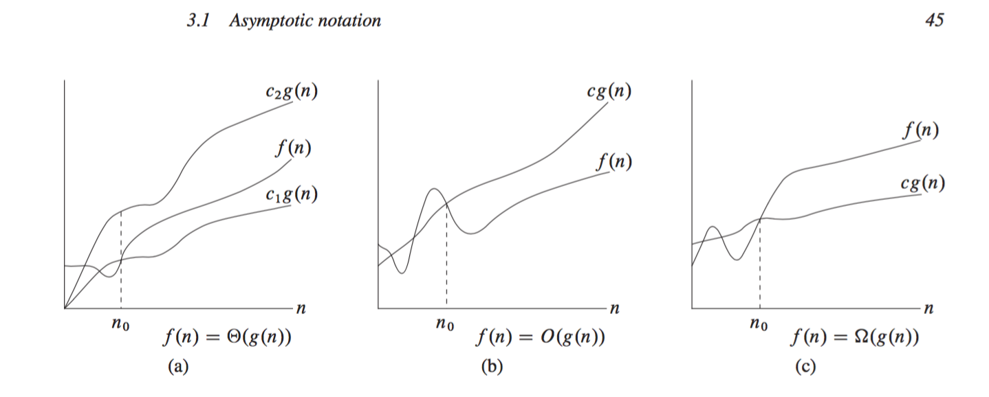
Before we start, let us briefly talk about asymptotic notation. Asymptotic notation is primarily used to describe the running times of algorithms, with each type of notation specifying a different bound (lower, upper, tight bound, etc.).

• Big-Theta: $\Theta$-notation bounds a function to within constant factors.

• Big-Oh: $O$-notation gives an upper bound for a function to within a constant factor.

• Big-Omega: $\Omega$-notation gives a lower bound for a function to within a constant factor.

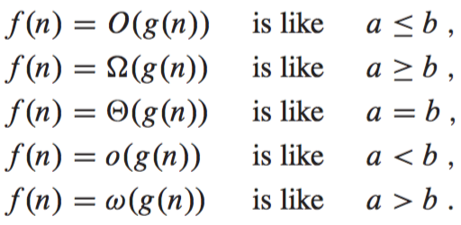
Small o-notation is used to denote an upper bound that is not asymptotically tight. The definitions of O-notation and o-notation are similar, but the main difference is that in $f(n) = O(g(n))$, the bound $0 <= f(n) <= c(g(n))$ holds for some constant c > 0, but in $f(n) = o(g(n))$, the bound $0 <= f(n) < c(g(n))$ holds for all constants c > 0. By analogy, $\omega$-notation (small omega) is to $\Omega$-notation (big omega) as o-notation is to O-notation. Cormen draws an analogy between the asymptotic comparison of two functions f and g and the comparison of two real numbers a and b as follows:

Naive matrix multiplication

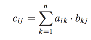
Let us start with two square matrices A and B which are both of size n by n. In the product C = A X B we define the entry $c_{ij}$, the entry in the $i^{th}$ row and the $j^{th}$ column of A, as being the dot product of the $i^{th}$ row of A with the $j^{th}$ column of B. Taking the dot product of vectors just means that you take the products of the individual components and then add up the results.

The following illustrations, taken from Introduction to Algortihms, Cormen et. al, sum this up nicely:

The first for loop at line 3 computes the entries of each row i, and within a given row i, the for loop from line 4 computes each of the entries $c_{ij}$ for each column j. Line 5 computes each entry $c_{ij}$ using the dot product, which was defined in the equation above. We can translate the pseudocode to Python code as follows:

import numpy as np
n,n = np.shape(A)
C = np.eye(n)
for i in range(n):
	for j in range(n):
		C[i][j] = 0
		for k in range (n):
			C[i][j] += A[i][k]*B[k][j]
return C

Each of the triply-nested for loops above runs for exactly n iterations, which means that the algorithm above has a runtime complexity of $\Theta(n^3)$. Roughgarden poses the following question:

So the question as always for the keen algorithm designer is, can we do better? Can we beat $n^3$ time for multiplying two matrices?

Cormen et al. note that:

You might at first think that any matrix multiplication algorithm must take $\omega(n^3)$ time, since the natural definition of matrix multiplication requires that many multiplications. You would be incorrect, however: we have a way to multiply matrices in $o(n^3)$ time. Strassen’s remarkable recursive algorithm for multiplying n by n matrices runs in $\Theta (n^{lg7})$ time.

So how is Strassen’s algorithm better? To answer that, we will first look at how we can apply the divide and conquer approach for multiplying matrices.

Divide and Conquer using Block Partitioning

Let us first assume that n is an exact power of 2 in each of the n x n matrices for A and B. This simplyifying assumption allows us to break a big n x n matrix into smaller blocks or quadrants of size n/2 x n/2, while also ensuring that the dimension n/2 is an integer. This process is termed as block partitioning and the good part about it is that once matrices are split into blocks and multiplied, the blocks behave as if they were atomic elements. The product of A and B can then be expressed in terms of its quadrants. This gives us an idea of a recursive approach where we can keep partitioning matrices into quadrants until they are small enough to be multiplied in the naive way.

The following equations from Cormen et al. illustrate this process:

In each of the 4 equations above we have two multiplications of n/2 x n/2 matrices that are then added together. A recursive, divide-and-conquer algorithm is then:

For multiplying two matrices of size n x n, we make 8 recursive calls above, each on a matrix/subproblem with size n/2 x n/2. Each of these recursive calls multiplies two n/2 x n/2 matrices, which are then added together. For the addition, we add two matrices of size $n^2/4$, so each addition takes $\Theta(n^2/4)$ time. We can write this recurrence in the form of the following equations (taken from Cormet et al.):

The master theorem is a way of figuring out the runtime complexity of algorithms that use the divide and conquer approach, where subproblems are of equal size. It was popularized by Cormen et al. Roughgarden refers to it as a “black box for solving recurrences”. The following equations are taken from his slides:

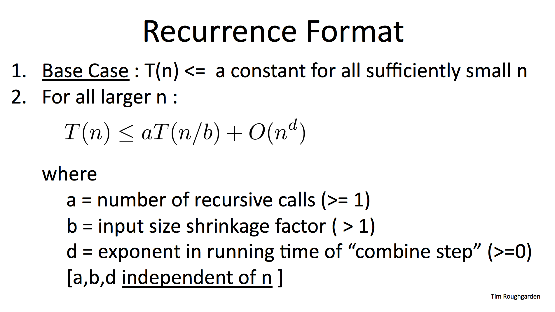
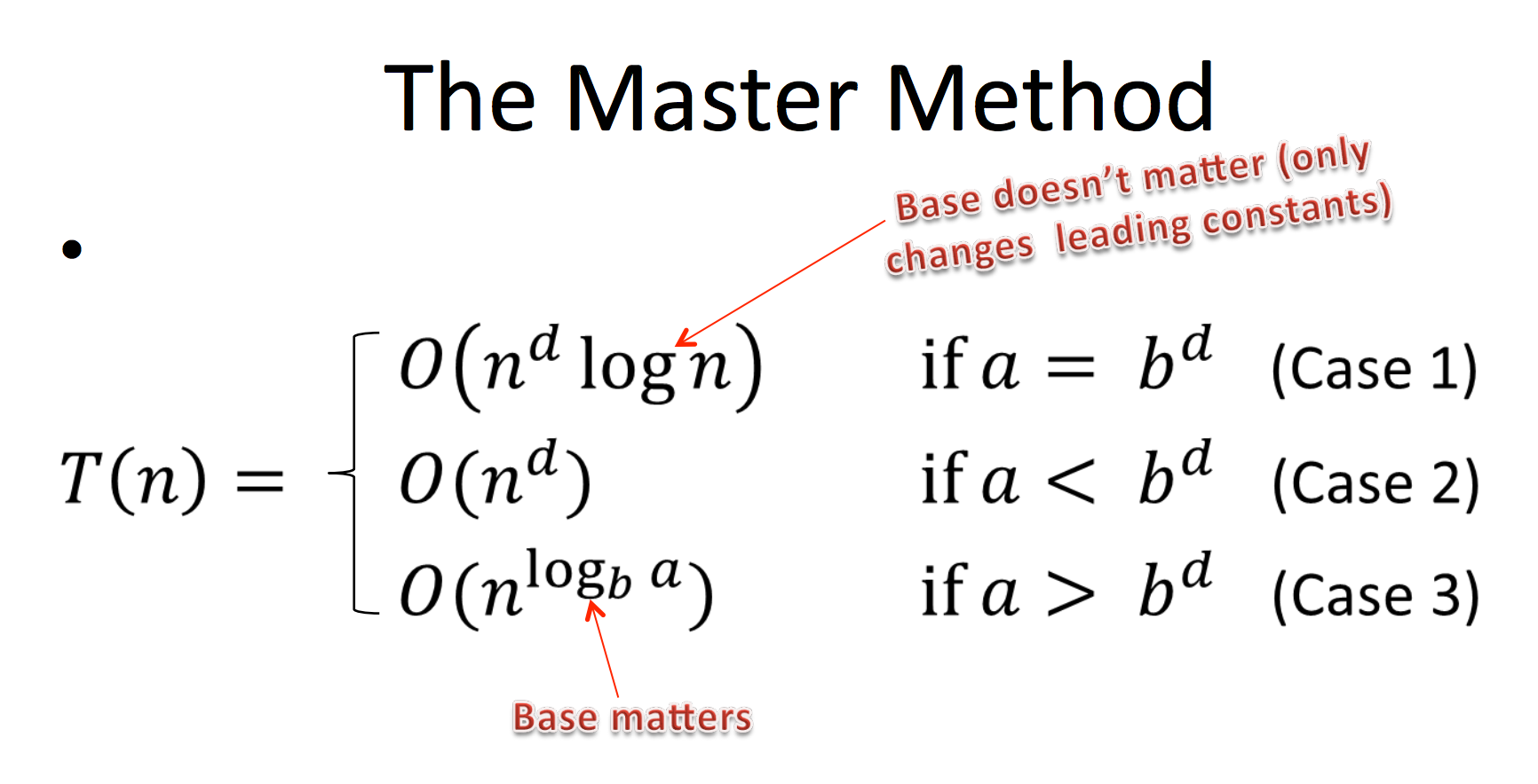
For our block partitioning approach, we saw that we had 8 recursive calls $(a=8)$, where each subproblem was of size n/2 x n/2 $(b=2)$. Outside of the recursive calls, we were performing additions that were of the order $n^2/4$ since each quadrant matrix had those many entries. So we were doing work of the order of $\Theta(n^2)$ outside of the recursive calls ($d=2$). This corresponds to case 3 of the master theorem since $a$ (8) is more than $b^d$ ($2^2 = 4$).

Using the master theorem, we can say that the runtime complexity is big $O(n^{log_b a})$, which is big $O(n^{log_2 8})$or big $O(n^3)$. This is no better than the straightforward iterative algorithm!

Strassen’s Algorithm

Strassen’s algorithm makes use of the same divide and conquer approach as above, but instead uses only 7 recursive calls rather than 8. This is enough to reduce the runtime complexity to sub-cubic time! See the following quote from Cormen:

The key to Strassen’s method is to make the recursion tree slightly less bushy. Strassen’s method is not at all obvious. (This might be the biggest understatement in this book.)

We save one recursive call, but have several new additions of n/2 x n/2 matrices. Strassen’s algorithm has four steps:

1) Divide the input matrices A and B into $n/2$ x $n/2$ submatrices, which takes $\Theta(1)$ time by performing index calculations.

2) Create 10 matrices $S_1$, $S_2$, $S_3$, … $S_{10}$ each of which is the sum or difference of two matrices created in step 1. We can create all 10 matrices in $\Theta(n^2)$ time.

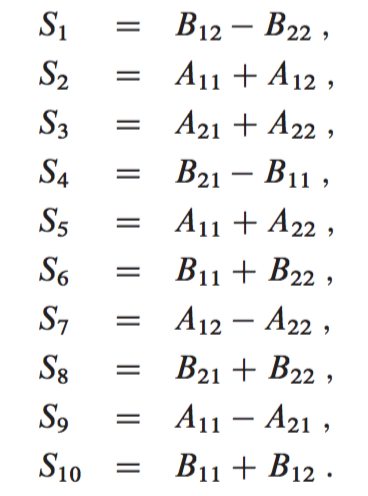3) Using the submatrices created from both of the steps above, recursively compute seven matrix products $P_1$, $P_2$, … $P_7$. Each matrix $P_{i}$ is of size n/2 x n/2.

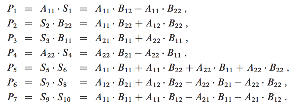
The products that we compute in our recursive calls are the ones from the middle column above. The right column just shows what these products equal in terms of the original submatrices from step 1.

4) Get the desired submatrices $C_{11}$, $C_{12}$, $C_{21}$, and $C_{22}$ of the result matrix C by adding and subtracting various combinations of the $P_i$ submatrices. These four submatrices can be computed in $\Theta(n^2)$ time.

Using the above steps, we get the recurrence of the following format:

In Strassen’s algorithm, we saw that we had 7 recursive calls $(a=7)$, where each subproblem or submatrix was of size n/2 x n/2 $(b=2)$. Outside of the recursive calls, we were performing work on the order of $\Theta(n^2)$ ($d=2$). This also corresponds to case 3 of the master theorem since $a$ (7) is more than $b^d$ ($2^2 = 4$).

However, unlike the first case, the runtime complexity here is big $O(n^{log_b a})$, which is big $O(n^{log_2 7})$ or big $O(n^{2.81})$. This beats the straightforward iterative approach & the regular block partitioning approach asymptotically!

Conclusion

We showed how Strassen’s algorithm was asymptotically faster than the basic procedure of multiplying matrices. Better asymptotic upper bounds for matrix multiplication have been found since Strassen’s algorithm came out in 1969. The most asymptotically efficient algorithm for multiplying n x n matrices to date is Coppersmith and Winograd’s algorithm, which has a running time of $O(n^{2.376})$.

However, in practice, Strassen’s algorithm is often not the method of choice for matrix multiplication. Cormen outlines the following four reasons for why:

1. The constant factor hidden in the $O(n^{log_2 7})$ running time of Strassen’s algorithm is larger than the constant factor in the > $O(n^{3})$ SQUARE-MATRIX-MULTIPLY procedure.

2. When the matrices are sparse, methods tailored for sparse matrices are faster.

3. Strassen’s algorithm is not quite as numerically stable as the regular approach. In other words, because of the limited precision of computer arithmetic on noninteger values, larger errors accumulate in Strassen’s algorithm than in SQUARE-MATRIX-MULTIPLY.

4. The submatrices formed at the levels of recursion consume space.

Cormen et al describe how the latter two reasons were mitigated around 1990. They state that the difference in numerical stability was overemphasized and although Strassen’s algorithm is too numerically unstable for some applications, it is within acceptable limits for others. In practice, fast matrix-multiplication implementations for dense matrices use Strassen’s algorithm for matrix sizes above a crossover point and they switch to a simpler method once the subproblem size reduces to below the crossover point. The exact value of the crossover point is highly system dependent. Crossover points on various systems were found to range from 400 to 2150.

In summary, even if algorithms like Strassen’s have lower asymptotic runtimes, they might not be implemented in practice due to issues with numerical stability. However, there can still be practical uses for them in certain scenarios, such as applying Strassen’s method when dealing with multiplications of large, dense matrices of a certain size.