Gradient Boosted Trees

In this post I will explore how Gradient Boosted Trees work. Gradient Boosting is a very popular and widely used (“off-the-shelf”) machine learning algorithm that often surpasses other algorithms in terms of predictive power. In almost every project and data challenge I have done at work and school, I have ended up using gradient boosting as my final model.

First I will start by explaining what boosting is and how it came into practice. I will then explore how gradient boosted trees work. I will use pseudocode along the way, and I will be referencing illustrations and notes from The Elements of Statistical Learning (ESL) by Friedman, Tibshirani, and Hastie. Initially, I will talk about boosting and loss functions from a binary classification perspective, but it can be extended to multi-class classification and regression problems as well.

Boosting - Introduction and AdaBoost

Boosting is a procedure that combines the outputs of many weak classifiers (usually decision trees) to produce a powerful “committee”. It is similar to other committee-based approaches like bagging. In bagging, we take an average of the predictions made by building models on bootstrapped (sampling with replacement) datasets. Since each model is trained on a different bootstrapped dataset, this approach can be parallelized.

Boosting, however, is a committee-based, sequential process that can’t be parallelized and which doesn’t use bootstrapping. AdaBoost.M1, a popular boosting algorithm due to Freund and Schapire (1997), works by training models on successive versions of the original data where observations that were misclassified by the previous model in the sequence are given higher weights than those that were correctly classified. Each model/tree in the sequence tries to correct for the errors made by the previous model. After a chosen number of modeling iterations, the final prediction is a weighted majority vote where each classifier is weighted according to its accuracy on the data it was trained on.

AdaBoost algorithm from ESL, Friedman et al:

We assume that the output variable is coded as Y ∈ {−1, 1}. This is the AdaBoost algorithm:

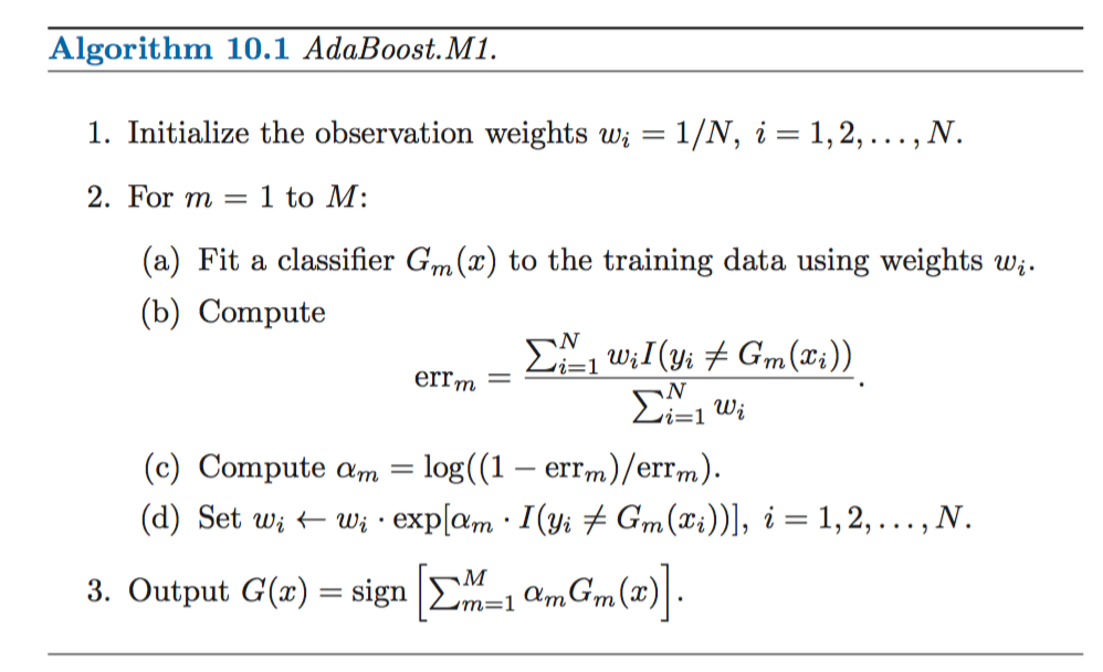
In practice, the classifiers or weak learners used in AdaBoost are stumps, which are decision trees with a single split.

In ESL, Friedman et al. show how AdaBoost.M1 is equivalent to forward-stagewise additive modeling using the exponential loss function.

Minimizing loss of additive model

Exponential loss

$$L(y, f (x)) = e^{(−y f (x))}$$

They also state why a stagewise rather than a stepwise approach is used:

For many loss functions $L(y,f(x))$ and/or basis functions $b(x;γ)$, this approach (stepwise) requires computationally intensive numerical optimization techniques. However, a simple alternative often can be found when it is feasible to rapidly solve the subproblem of fitting just a single basis function. Forward stagewise modeling approximates the solution by sequentially adding new basis functions to the expansion without adjusting the parameters and coefficients of those that have already been added.

Hence, we can think of boosting as a numerical optimization problem where we have to minimize the loss using stagewise procedures. One weak learner is added at a time, without changing the previously computed parameters and coefficients of earlier models in the sequence.

Gradient Boosted Trees

Gradient Boosted Trees are an ensemble of decision trees that are built in a stagewise fashion, allowing optimization of any differentiable loss function. In fact, for binary classification problems using the exponential loss function, Gradient Boosting is equivalent to AdaBoost.

When a tree is added one at a time in the stagewise approach, we use a gradient descent procedure to minimize the loss. We do this by parametrizing the trees and moving in the direction indicated by gradient descent, reducing the residual loss at that step. This approach is referred to as functional gradient descent.

Tree parameters and approach

Decision trees work by partitioning the feature space into disjoint regions $R_{j} , j . . . J$. For x in particular region $R_j$ the value of T(x) is constant. A tree can be formally expressed as:

$$T(x,\gamma) = \sum_{j=1}^{J} \beta_{j} I(x ∈ R_j)$$

where $I(x ∈ R_j)$ is an indicator variable that takes the value of 1 if x belongs to region $R_j$, or 0 otherwise.

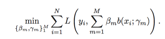
The boosted tree model is a sum of M trees

$$f_{M} (x) = \sum_{m=1}^{M} T(x,\gamma_{m})$$

induced in a forward stagewise manner. At each step $m$, we first find the regions $\{ R_{jm} \}_{m=1}^J$ by solving

$$\gamma_m = arg min_\gamma \sum_{i=1}^{N} L(y_i,f_{m−1}(x_i)+ T(x_i,\gamma))$$

Given the regions $R_{jm}$, finding the optimal constants for each region can be done by

$$β_{jm} = arg min_\beta \sum_{x_{i} ∈ R_{jm}}^{} L(y_i, f_{m−1}(x_i) + β))$$

Gradient Boosted Trees for Regression with Squared Loss

To make the problem more clear, let’s consider the case of the squared loss for regression.

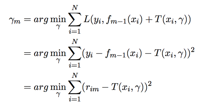
where $r_{im} = y_{i} − f_{m−1} (x_i)$ is the residual for observation $i$ at iteration $m$. This problem is a standard regression tree problem that can be solved using CART or any other regression tree method.

$$β_{jm} = arg min_\beta \sum_{x_{i} ∈ R_{jm}}^{} L(y_i, f_{m−1}(x_i) + β)$$ $$= arg min_\beta \sum_{x_{i} ∈ R_{jm}}^{} (r_{im}-β)^2$$

This last problem has an analytical solution where $β$ is the average of $r_{im}$ over $R_{jm}$.

Algorithm and other loss functions (illustrations taken from ESL)

We have seen how gradient boosted trees work for regression using a squared loss. We can also use different loss criteria; the following illustration outlines the generic gradient tree-boosting algorithm for regression:

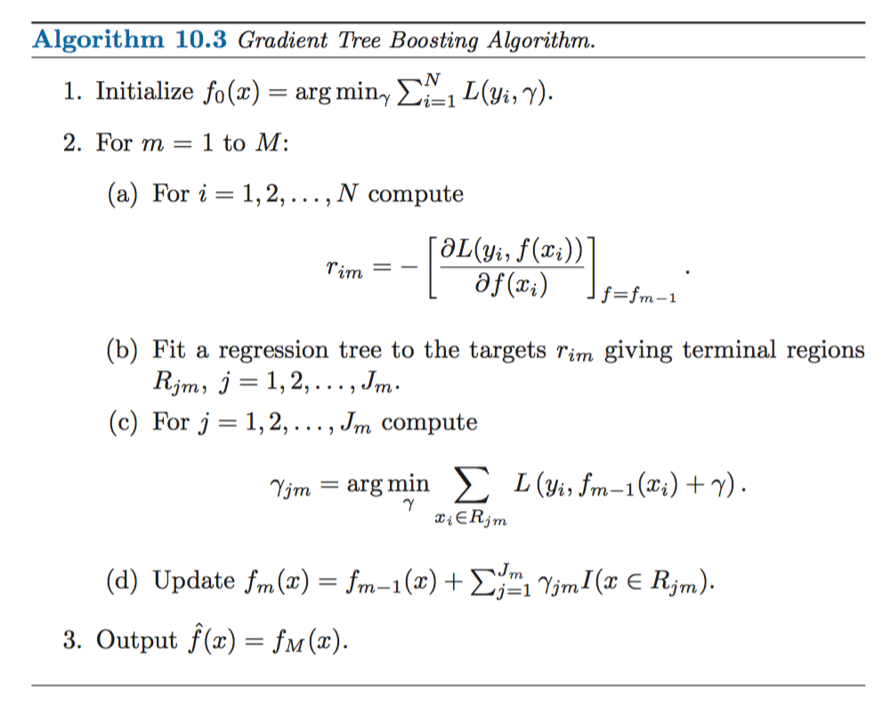
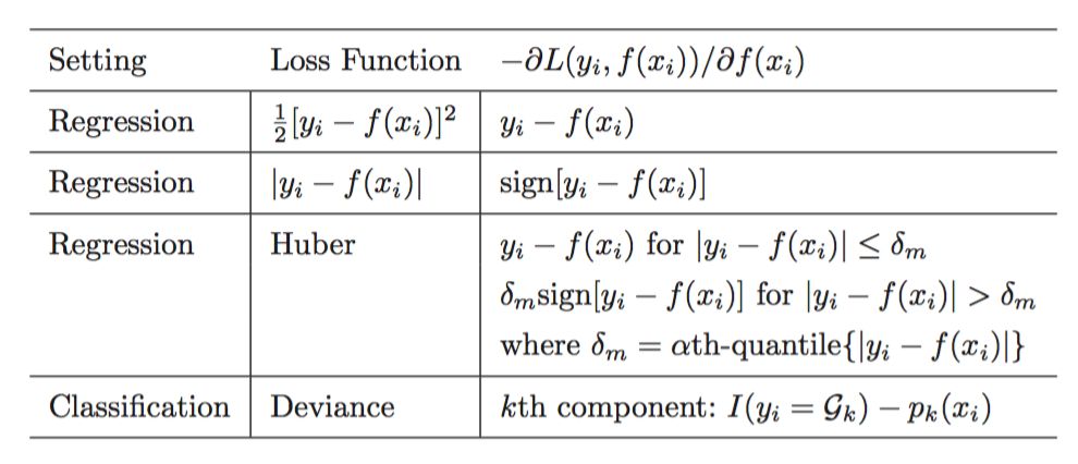
Specific algorithms are obtained by inserting different loss criteria $L(y,f(x))$. Gradients for commonly used loss functions are shown below:

Tree constraints and regularization

There are certain tree constraints that we can choose to tune:

• Number of trees, M - The main tuning parameter, it is often picked by monitoring the performance on a separate validation set, and then stopping once performance starts to decrease.
• Tree depth - Deeper trees capture more interactions and complexities, usually a depth between 4 and 8 suffices.
• Number of nodes
• Minimum loss reduction

We can also use L1 or L2 regularization terms to avoid overfitting.